plot() visualizes the relationship between a PCO axis and the vertebra or between pairs of PCO axes.
Usage
# S3 method for class 'regions_pco'
plot(x, pc_y = 1, pc_x = NULL, ...)
Arguments
- x
a
regions_pcoobject; the output of a call tosvdPCO().- pc_y, pc_x
number; PC score indices for the y- and x-axes, respectively.
pc_xcan beNULL.- ...
arguments passed to
ggplot2::geom_text()whenpc_xis notNULL. Ifscoresis supplied as an argument, it will replacepc_yif unspecified.
Details
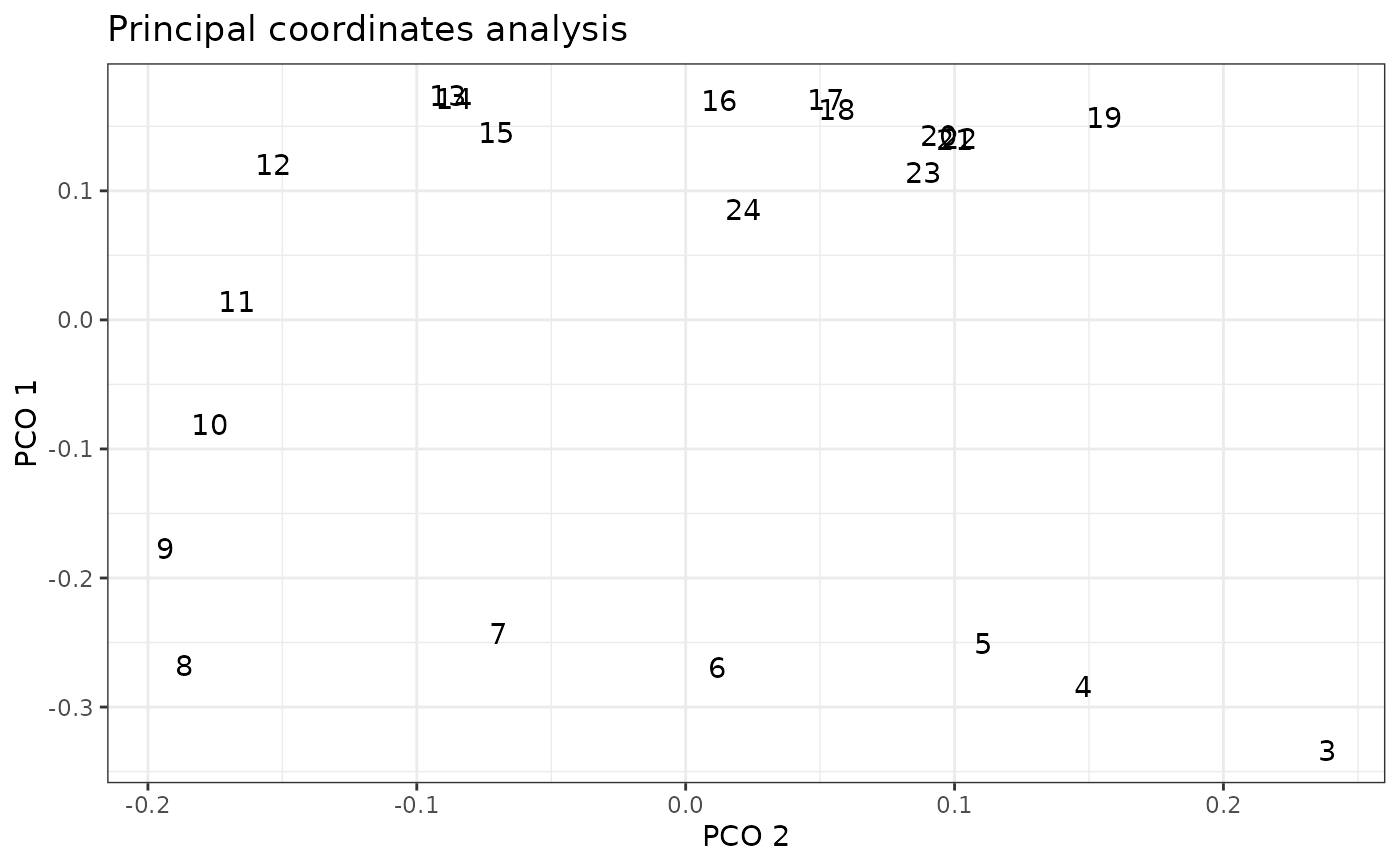
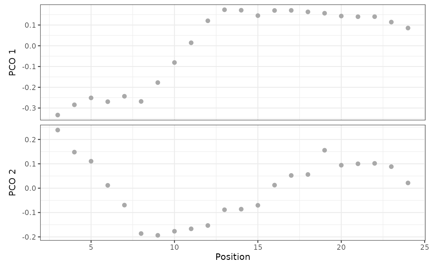
When pc_x is NULL (the default), plot() will display a scatterplot of the PCO axis identified by pc_y and vertebra position using ggplot2::geom_point(). This plot is similar to that generated by plotsegreg(). Otherwise, plot() uses ggplot2::geom_text() to identify vertebrae positions in the space corresponding to the requested PCOs.
See also
svdPCO() for generating the PCO scores. plot.regions_sim() for plotting PCO scores against vertebra position for simulated PCOs. plotsegreg() for plotting PCO scores against vertebra position after selecting breakpoints for a segmented regression.
Examples
data("alligator")

alligator_data <- process_measurements(alligator,
                                       pos = "Vertebra")

# Compute PCOs
alligator_PCO <- svdPCO(alligator_data,
                        metric = "gower")

alligator_PCO
#> - Scores:
#>
#>    PCO.1   PCO.2    PCO.3    PCO.4    PCO.5    PCO.6    PCO.7   PCO.8    PCO.9
#> 1 -0.334  0.2386  0.03426 -0.10271 -0.04904 -0.04760 -0.03210 -0.0341 -0.00170
#> 2 -0.284  0.1480 -0.02979 -0.01372  0.06610 -0.03238  0.05522  0.0245  0.01972
#> 3 -0.251  0.1106 -0.07088  0.05289  0.04260 -0.02385 -0.03003  0.0160 -0.03045
#> 4 -0.269  0.0116 -0.09275  0.07987 -0.00401  0.00907  0.00464  0.0231 -0.00295
#> 5 -0.243 -0.0695 -0.04831  0.01709 -0.05224  0.06285 -0.02271  0.0222  0.00941
#> 6 -0.268 -0.1863  0.00344 -0.00869 -0.00536  0.06317 -0.02513 -0.0205  0.02758
#>      PCO.10   PCO.11    PCO.12   PCO.13    PCO.14   PCO.15   PCO.16    PCO.17
#> 1  0.018670  0.00486  0.000221  0.00457  0.000393 -0.00198 -0.00860  0.000428
#> 2 -0.036114  0.00829 -0.027648 -0.01465  0.004165 -0.00981  0.00182 -0.003757
#> 3  0.000191 -0.02548  0.040047  0.00938  0.009774  0.02548  0.01119  0.007634
#> 4  0.025317  0.01864  0.003402  0.01498 -0.021639 -0.03377 -0.00674 -0.005831
#> 5  0.020205 -0.01407 -0.032932 -0.04248  0.003092  0.01802 -0.00649  0.005655
#> 6 -0.045238  0.02653  0.020049  0.02394  0.007392  0.00588  0.00227 -0.001655
#>      PCO.18   PCO.19    PCO.20    PCO.21
#> 1  0.001471  0.00337 -0.001435  0.000816
#> 2 -0.008612 -0.00597  0.001839  0.002614
#> 3 -0.000183 -0.00604  0.002491 -0.002083
#> 4  0.012116  0.01142 -0.002113 -0.001988
#> 5 -0.001655 -0.00516  0.002234 -0.001151
#> 6 -0.011215  0.00492 -0.000682  0.002172
#> (First 6 of 22 rows displayed.)
#>
#> - Eigenvalues:
#>
#>  [1] 7.81e-01 3.39e-01 1.59e-01 4.17e-02 2.94e-02 2.73e-02 1.86e-02 1.32e-02
#>  [9] 1.29e-02 1.17e-02 8.97e-03 8.39e-03 7.81e-03 6.20e-03 5.88e-03 2.85e-03
#> [17] 2.12e-03 2.00e-03 1.38e-03 9.43e-04 3.79e-04 8.08e-17

# Plot PCOs against vertebra index
plot(alligator_PCO, pco_y = 1:2)


# Plot PCOs against each other
plot(alligator_PCO, pco_y = 1, pco_x = 2)
# Plot PCOs against each other
plot(alligator_PCO, pco_y = 1, pco_x = 2)