Calculates distance matrix from raw data, then conducts a PCO ordination using a
single value decomposition (SVD). This differs from other PCO functions which use stats::cmdscale() and rely on a
spectral decomposition.
Arguments
- x
a
regions_dataobject; the output of a call toprocess_measurements().- metric
string; the distance matrix calculation metric. Allowable options include those support by
cluster::daisy(), which are"euclidean","manhattan", or"gower". Default is"gower". Abbreviations allowed.- scale
logical; whether to scale the variables prior to including them in the PCO estimation. Default isTRUE, which is especially advisable when using the bootstrap to select the number of PCOs to use in downstream analyses. Passed to thestandargument ofcluster::daisy(). Ignored ifmetric = "gower".
Value
A regions_pco object, which contains eigenvectors in the scores component and eigenvalues in the eigen.val component. The original dataset is stored in the data attribute.
See also
plot.regions_pco()for plotting PCO axescluster::daisy(), which is used to compute the distance matrix used in the calculationstats::cmdscale()for a spectral decomposition-based implementation
Examples
data("alligator")
alligator_data <- process_measurements(alligator,
pos = "Vertebra")
# Compute PCOs
alligator_PCO <- svdPCO(alligator_data,
metric = "gower")
alligator_PCO
#> - Scores:
#>
#> PCO.1 PCO.2 PCO.3 PCO.4 PCO.5 PCO.6 PCO.7 PCO.8 PCO.9
#> 1 -0.334 0.2386 0.03426 -0.10271 -0.04904 -0.04760 -0.03210 -0.0341 -0.00170
#> 2 -0.284 0.1480 -0.02979 -0.01372 0.06610 -0.03238 0.05522 0.0245 0.01972
#> 3 -0.251 0.1106 -0.07088 0.05289 0.04260 -0.02385 -0.03003 0.0160 -0.03045
#> 4 -0.269 0.0116 -0.09275 0.07987 -0.00401 0.00907 0.00464 0.0231 -0.00295
#> 5 -0.243 -0.0695 -0.04831 0.01709 -0.05224 0.06285 -0.02271 0.0222 0.00941
#> 6 -0.268 -0.1863 0.00344 -0.00869 -0.00536 0.06317 -0.02513 -0.0205 0.02758
#> PCO.10 PCO.11 PCO.12 PCO.13 PCO.14 PCO.15 PCO.16 PCO.17
#> 1 0.018670 0.00486 0.000221 0.00457 0.000393 -0.00198 -0.00860 0.000428
#> 2 -0.036114 0.00829 -0.027648 -0.01465 0.004165 -0.00981 0.00182 -0.003757
#> 3 0.000191 -0.02548 0.040047 0.00938 0.009774 0.02548 0.01119 0.007634
#> 4 0.025317 0.01864 0.003402 0.01498 -0.021639 -0.03377 -0.00674 -0.005831
#> 5 0.020205 -0.01407 -0.032932 -0.04248 0.003092 0.01802 -0.00649 0.005655
#> 6 -0.045238 0.02653 0.020049 0.02394 0.007392 0.00588 0.00227 -0.001655
#> PCO.18 PCO.19 PCO.20 PCO.21
#> 1 0.001471 0.00337 -0.001435 0.000816
#> 2 -0.008612 -0.00597 0.001839 0.002614
#> 3 -0.000183 -0.00604 0.002491 -0.002083
#> 4 0.012116 0.01142 -0.002113 -0.001988
#> 5 -0.001655 -0.00516 0.002234 -0.001151
#> 6 -0.011215 0.00492 -0.000682 0.002172
#> (First 6 of 22 rows displayed.)
#>
#> - Eigenvalues:
#>
#> [1] 7.81e-01 3.39e-01 1.59e-01 4.17e-02 2.94e-02 2.73e-02 1.86e-02 1.32e-02
#> [9] 1.29e-02 1.17e-02 8.97e-03 8.39e-03 7.81e-03 6.20e-03 5.88e-03 2.85e-03
#> [17] 2.12e-03 2.00e-03 1.38e-03 9.43e-04 3.79e-04 8.08e-17
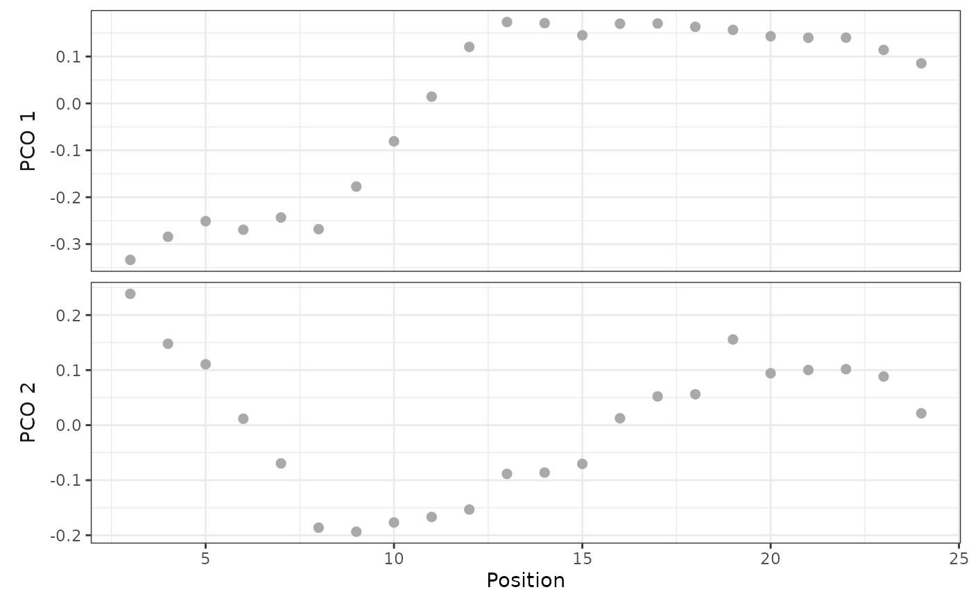
# Plot PCOs against vertebra index
plot(alligator_PCO, pco_y = 1:2)
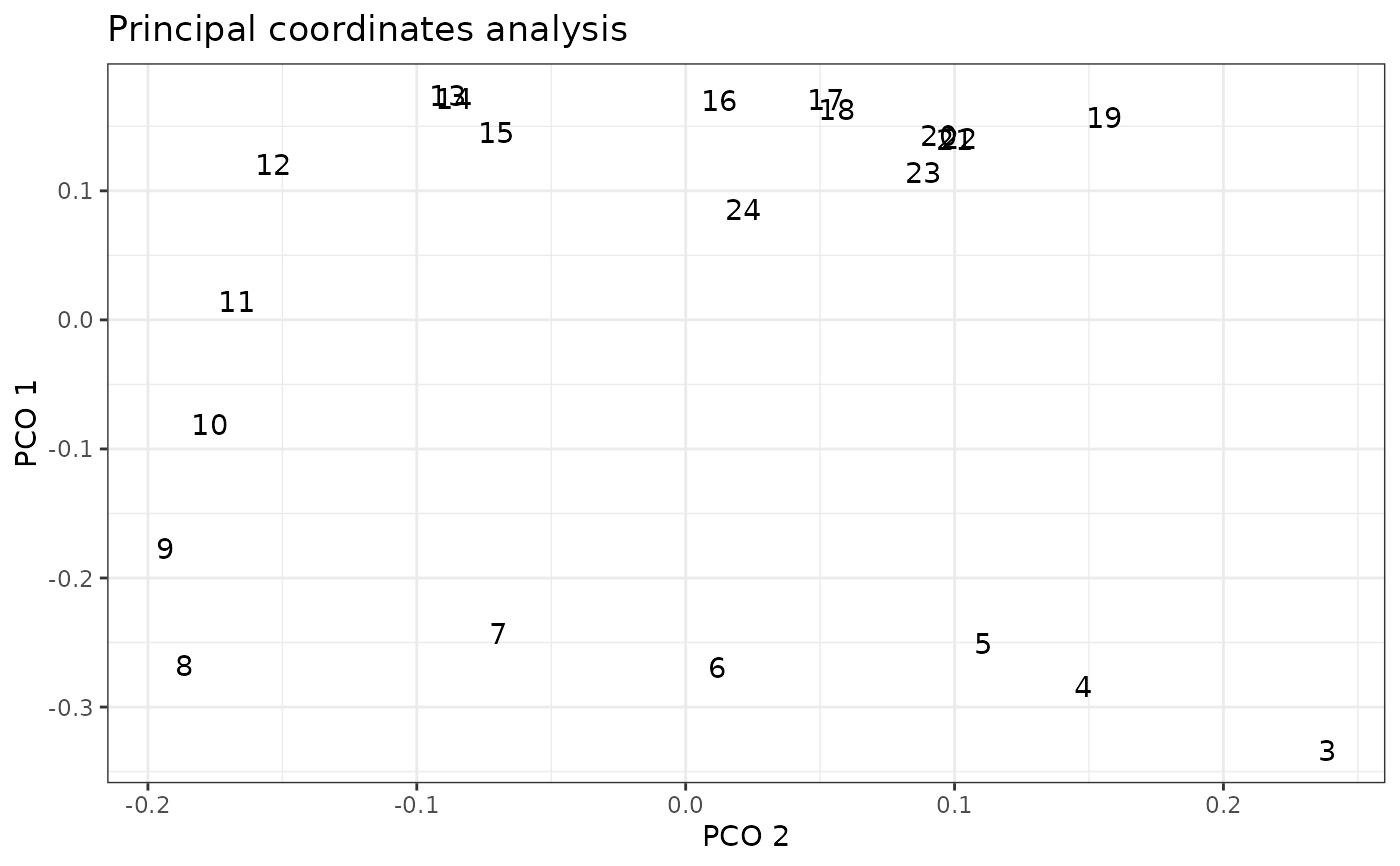
 # Plot PCOs against each other
plot(alligator_PCO, pco_y = 1, pco_x = 2)
# Plot PCOs against each other
plot(alligator_PCO, pco_y = 1, pco_x = 2)