Calculate PCO loadings

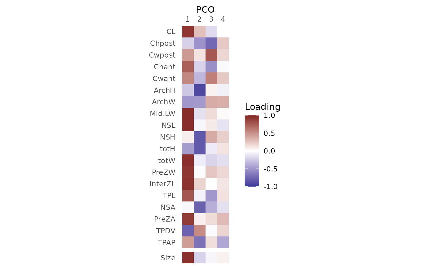
PCOload() computes the loadings for each principal coordinates (PCOs) analysis score, which are the correlations between the features used to compute the PCOs and the PCOs.

Usage

PCOload(x, scores)

# S3 method for class 'regions_pco_load'
plot(x, ...)

Arguments

x

for PCOload(), a regions_pco object; the output of a call to svdPCO(). For plot(), a regions_pco_load object.

scores

a numeric vector containing the indices of the desired scores.

...

ignored.

Value

PCOload() returns a regions_pco_load object, which is a matrix with a column for each PCO score requested and a row for each variable in the original dataset; values indicate the correlation between each variable and each PCO score. plot() returns a ggplot object, which can be manipulated using ggplot2 syntax, that displays the loadings visually.

Details

The loadings for a constructed variable, vert.size, are also computed and displayed. This is computed as the mean of the features for each vertebra. This function is not suitable for geometric morphometric data.

See also

svdPCO() for computing the PCOs; plot.regions_pco() for visualizing the correlations between PCO scores.

Examples

data("alligator")

alligator_data <- process_measurements(alligator,
                                       pos = "Vertebra")

# Compute PCOs
alligator_PCO <- svdPCO(alligator_data)

# Compute PCO loadings
loadings <- PCOload(alligator_PCO, scores = 1:4)
loadings
#> - PC loadings:
#> 
#>            PC.1    PC.2     PC.3      PC.4
#> CL       0.9214  0.2850 -0.17096  0.000379
#> Chpost  -0.2163 -0.5189 -0.74326  0.240596
#> Cwpost   0.4554  0.1168  0.75907  0.175309
#> Chant    0.7288 -0.2063 -0.53556 -0.028160
#> Cwant    0.5402 -0.3457  0.57294  0.238653
#> ArchH   -0.2635 -0.9168  0.05630 -0.065128
#> ArchW   -0.4975 -0.4906  0.36905  0.357137
#> Mid.LW   0.9664 -0.1441  0.15972  0.021917
#> NSL      0.9580 -0.0427  0.09103 -0.127765
#> NSH      0.0773 -0.8326  0.37861  0.212040
#> totH    -0.4753 -0.8241 -0.09257  0.121630
#> totW     0.9532 -0.0821 -0.20079 -0.150651
#> PreZW    0.9248 -0.0133  0.25234  0.171984
#> InterZL  0.9406  0.1956 -0.00413  0.114973
#> TPL      0.7768 -0.0630 -0.50157  0.132715
#> NSA     -0.0383 -0.7876 -0.38165 -0.145363
#> PreZA    0.8968  0.0704  0.15874  0.304670
#> TPDV    -0.7728  0.5232 -0.02010  0.189908
#> TPAP     0.4419 -0.6879  0.14413 -0.418512
#> 
#>  - Corr w/ vertebra size:
#> 
#>            PC.1   PC.2    PC.3   PC.4
#> vert.size 0.952 -0.207 -0.0441 0.0624

# Plot loadings
plot(loadings)